
Viscosity Measurements of Transparent Glycerol-Water Mixtures Using Diffusing Wave Spectroscopy
Related Product
DWS RheoLab™
The DWS RheoLab™ is a contact-free rheometer. It provides access to the sample's viscoelastic properties over an unmatched frequency range and enables the study of textures and microstructures while requiring only small sample volumes.
Introduction
Diffusing Wave Spectroscopy (DWS) is a powerful optical technique primarily used to study the rheological properties of turbid samples. The method is based on the analysis of the fluctuations of laser light that is scattered multiple times within a sample [1,2]. The DWS RheoLab from LS Instruments is a versatile tool to conduct such measurements.
Because DWS requires sufficient turbidity to ensure strong multiple scattering of laser light, samples such as creams, milk, yoghurt, lotions, shampoos, paints, and ceramics are well suited. However, if the sample is transparent, some sample preparation is required prior to measurement.
The purpose of this application note is to show how one can prepare a transparent sample by adding tracer particles to obtain sufficient turbidity for DWS measurements. As a model system, we use mixtures of glycerol with water at different mixing ratios and compare the measured viscosities with tabulated (published) values. Moreover, we explain how one can measure the transport mean free path l* over an extended range of turbidity. This is the distance after which a scattered photon has totally lost its original propagation direction. It thus indicates how turbid a sample is. The smaller l* is, the stronger the scattering. Accurate values of l* are necessary not only for extracting viscoelastic information from DWS measurements but also for many other applications. It is the most important optical parameter for turbid samples.
Sample Preparation
Mixtures with different ratios of glycerol and water were prepared. Tracer particles, consisting of polystyrene beads with a diameter of 980 nm dispersed in water, were added. We used a tracer particle concentration of approximately 2 wt% (solid content) for all samples. Table 1 summarizes the different samples S1 to S5.
The choice of the tracer particle concentration is connected to the cuvette size. The cornerstone of accurate DWS measurements is ensuring the applicability of the diffusion approximation which requires that L≥ 5 l*, where L is the thickness of the cuvette [1]. In the case of dilute systems l* is inversely proportional to the tracer particle concentration. Furthermore, l* is dependent on the refractive index of the solvent nsolv (see Table 1). In our system, an increase in glycerol concentration leads to an increase in nsolv which decreases the optical contrast of the tracer particles. Thus, an increase in the glycerol concentration yields an increased l*.
|
sample |
[glycerol] |
nsolv |
CR |
l* |
η |
|
- |
wt.% |
- |
kHz |
µm |
mPa·s |
|
S1 |
30.9 |
1.372 |
346 |
224 |
3.12±0.03 |
|
S2 |
48.6 |
1.396 |
409 |
283 |
6.20±0.08 |
|
S3 |
64.7 |
1.419 |
470 |
357 |
16.8±0.6 |
|
S4 |
77.9 |
1.439 |
506 |
407 |
55.9±1 |
|
S5 |
86.5 |
1.453 |
539 |
459 |
183±5 |
Table 1. Properties of the samples S1 to S5: weight fraction of glycerol in the solvent, refractive index nsolv of the solvent from tables [3], count-rate CR measured with DWS RheoLab, obtained l* based on CR, viscosity η measured with DWS RheoLab at a temperature of 20°C.
Determination of l*
The transport mean free path l* can be calculated based on Mie-theory (e.g. implemented in the web-based scattering calculator [4]). For accurate results, however, the precise particle concentration must be known. One must also pay attention to use volume fraction (not weight fraction) for the calculation!
To circumvent these problems, the DWS RheoLab offers the possibility to measure l* based on a reference sample thereby eliminating the need to know the concentration of the scattering particles. The reference sample must consist of dispersed monodisperse particles of well-known size (e.g. determined by static or dynamic light scattering or purchased from a reliable particle supplier). Typically one will use the same or similar particles at approximately the same concentration for both the reference and the sample. To determine l* the following equation can then be applied:
,
where the count rates CR are simply the number of photons per second measured in transmission by the optical detector of the DWS RheoLab. The count rates of the sample CRsample and the reference CRref must be determined for cuvettes of equal thicknesses L and a constant setting of the optical attenuator.
This approach is accurate under the condition that L≥ 5l*. Furthermore CRsample and CRref may not differ by more than 20 %. However, in our example, the resulting CRs range from 346 to 539 kHz for S1 to S5 (see Table 1) because of the different refractive index of each sample. We thus choose a set of 5 reference samples, with different concentrations of polystyrene beads (diameter of 980 nm) dispersed in water to never have a difference of more than 20 % in CR between sample and reference. Table 2 summarizes the properties of the different reference samples R1 to R5.
|
reference sample |
[tracer particle] |
CR |
l* |
|
- |
wt% |
kHz |
µm |
|
R1 |
2.07 |
271 |
174 |
|
R2 |
1.70 |
326 |
210 |
|
R3 |
1.32 |
399 |
276 |
|
R4 |
0.95 |
497 |
392 |
|
R5 |
0.69 |
574 |
522 |
Table 2. Properties of the reference samples R1 to R5: tracer particle concentration, count rate CR and transport mean free path l* measured with DWS RheoLab.
The use of the appropriate reference sample (R1 to R5) for each sample (S1 to S5) is sufficient to reach an accuracy of about 10 % in the determination of l*. However, we can further increase the accuracy by using an interpolation scheme. The measured count rates CR and transport mean free paths l* allow us to establish the calibration curve shown in Figure 1, which is a fit of the five data points from the reference samples with a second order polynomial.
Based on this calibration curve we determine l* of S1 to S5 with interpolation (see Table 1). Note that this curve holds only for a given laser intensity. The intensity of the laser may not be changed during the measurements on R1 to R5 and S1 to S5. In most cases, a single reference sample is sufficient when measuring several samples.
Only when the count rate (i.e. l*) varies over a wide range among the different samples, as in this particular case, several reference samples are recommended.
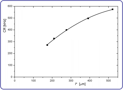
Figure 1. Calibration curve obtained from the reference samples R1 to R5 (squares) and a fit (line) using a second order polynomial.
Determination of the Viscosity
We now have all the parameters needed to extract the viscosity η from the measured correlation functions of the samples S1 to S5. This analysis can be done using the DWS RheoLabsoftware, where the correlation functions are loaded and the parameters nsolv, l* and tracer particle size are edited. In the "Analysis" tab in the user interface the frequency dependent storage and loss moduli can be calculated and extracted. The viscosity η is related to the loss modulus G’' via:
,
where ω is the frequency. Figure 2 shows the obtained viscosity η using Equation 2 and G" given by the DWS RheoLabsoftware. The results show basically no frequency dependency as expected for a Newtonian system. Moreover, the results demonstrate that the accessible frequency range depends on the viscosity. This range is shifted to higher frequencies for lower viscosities and can be tuned to some extent by modifying L and/or l*.
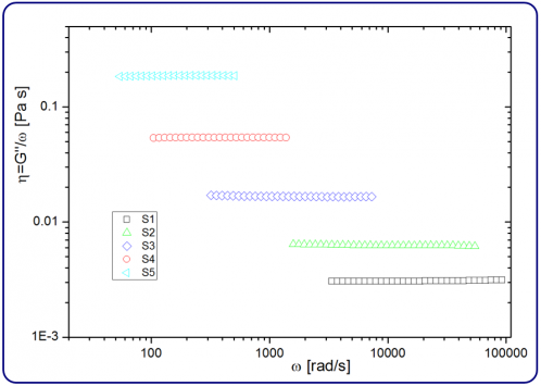
Figure 2. The measured viscosity η of the samples S1 to S5. The values are independent of the frequency as expected for a Newtonian system.
From these results, we calculate the mean values for η over the frequency range (see Table 1). Figure 3 shows the obtained viscosities of S1 to S5 (circles) and compares with tabulated values (line) for the viscosity of glycerol-water mixtures. Error bars represent the standard deviation of 6 independent measurements and an estimated error in glycerol concentration of 1 wt%. The measured values are on the order of 10 % larger than the tabulated values (except S1 and S5, which are 20 % larger).
The constant shift towards higher values suggests a deviation of the glycerol concentration of the samples (e.g. due to erroneous glycerol concentration of the stock solution or evaporation). The experimental data are consistent with an error of about 3 wt% in the glycerol concentration.
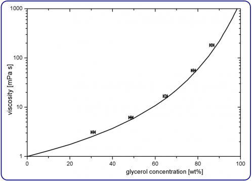
Figure 3. Viscosity versus the glycerol concentration. The experimental values (circles) correspond to S1 to S5 and the line represents tabulated values [5].
Conclusion
We applied DWS to initially transparent glycerol-water-mixtures. Tracer particles were added to ensure sufficient turbidity. This allowed us to access viscosities over a wide range (1:200) depending on the glycerol content of the sample. The measured values are highly reproducible and independent of the frequency as expected for a Newtonian system and agree well with the literature. This demonstrates that DWS microrheology is well suited for the quantitative characte-rization of non-turbid systems if tracer particles are added.
References
[1] D.A. Weitz, and D.J. Pine, Diffusing-Wave Spectroscopy. In Dynamic Light Scattering; Brown, W., Ed.; Oxford University Press: New York, 652-720 (1993).
[2] D. Lopez-Diaz, and R. Castillo, Microrheology of solutions embedded with thread-like supramolecular structures, Soft Matter 7, 5926–5937 (2011).
[3] W. M. Haynes, Handbook of Chemistry and Physics, 81st Edition, CRC press (2004).
[4] Mie-theory based scattering calculator for suspension of spherical particles, http://www.lsinstruments.ch/mie_calculator/
[5] N.E. Dorsey, The Properties of Ordinary Water Substance, New York (1940).