LS Instruments | Multi-τ Correlator

Multi-τ Correlator

To obtain high measurement accuracy with a linear correlator, a very short sampling time, usually of the order of 10 ns, is required. Under these constraints, a total measurement duration of even 1 s would require a dynamic range of 10⁸ s and a corresponding number of 10⁸channels, which is technically unfeasible. To circumvent the issue, other schemes, based on non-linearly spaced time sampling, have been proposed [1], among which the so-called Multi- $\tau$ method is surely the most widely adopted. The Multi-τarchitecture consist of a sequence of elementary linear correlator blocks.

Each one is characterized by a sampling time doubled compared to the correlator one level up in the hierarchical structure. This technique, by establishing a quasi-logarithmic time grid, combines the fine timing resolution of the linear correlator with the advantage of a large dynamic range. A general schematic of the Multi- $\tau$ algorithm, as implemented in the LSI Correlator, is illustrated in the figure below. The pulse train emitted by the APD is firstly acquired and pulses are subsequently counted over an initial sampling time. Each m-th correlator is clocked via its sampling time 2^mΔt.

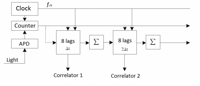
Multi-tau correlator architecture
Muti-tau correlator architecture

Within this architecture, effectively constituted of a cascade of linear correlator blocks, when a new sample is ready (see the figure from left to right), it is transferred to the first correlator that computes the correlation function for 8 correlation channels. Once two samples have been processed, they are accumulated and sent to the next correlator which in turn, repeats the same operation.

The Multi- $\tau$ framework based on a logarithmic spacing of lag-time axis holds the ability to cover extremely large extremely large lag time ranges with a small number of channels without incurring in substantial sampling errors. Such errors, in fact, can be kept negligibly small by using lag times larger than the sampling time. Specifically, a factor $\tau_k/\Delta t = 8$ suffices to reduce the absolute distortions below the typical statistical accuracy in PCS measurements [1].

Normalization

Normalization of the numerical correlation function consists in the baseline subtraction and division by the square of count rate estimator, hence yielding the normalized intensity correlation function:

$g_2(\tau_k)= \frac{G(\tau_k)-n_0^2}{n_0^2}$

Where $n_0=\sum_{i=1}^N n(t_i)/N$ is the count rate estimator. This procedure requires the addition of an extra monitor channel for computing the total photoelectron pulses detected, $n_0$ .

In order to obtain better noise performance, especially at large lags and sample times, two additional normalization schemes have been proposed [1]. In particular, if $n_k=\sum_{i=1}^{N-k} n(t_i)/N$ is the partial sum of those samples crossing the correlator channel k, the symmetric and compensated normalizations read respectively:

$g_2^{sym}(\tau_k)= \frac{G(\tau_k)-n_0n_k}{n_0n_k},$
and

$g_2^{com}(\tau_k)= \frac{G(\tau_k)-n_0n_k}{n_0^2}.$

Both advanced schemes evidently require extra monitor channels, for each single correlator channel and for each sampling time $2^m\Delta t$ .

[1] Schatzel K. Dynamic Light Scattering: The Method and some Applications. Ed. Clarendon Press, Oxford University Press, 1993.
[2] W. Liu, J. Shen, and X. Sun. Design of multiple-tau photon correlation system implemented by FPGA. Embedded Software and Systems, 2008. ICESS 08.

Previous Chapter