LS Instruments | Complex fluids

Complex fluids

Under shear, viscosity η is the fluid friction in relation to a displacement. It is thus the ratio between the shear stress and the shear rate: $\eta=\sigma \dot{\gamma}$ . The rheological fingerprint of a fluid is given by the shear stress dependent shear rate $\sigma ( \dot{\gamma})$ , which is called the flow curve.

In a Newtonian fluid, σ grows linearly with $\dot{\gamma}$ . This means that the viscosity is constant, it varies only with the temperature and does not depend on the motion the liquid is subjected to. Thus, when there is no linear σ-dependence on $\dot{\gamma}$ , the fluid is called non-Newtonian. In this case, the viscosity is a function of the applied motion: $\sigma=\eta \dot{\gamma}$ .

paints, discover their incredible rheological properties

A non-Newtonian fluid can be either shear thinning or shear thickening, like wall paints or cornstarch dissolved in water, respectively. In the former case, σ growths is less than linear (η decreases with $\dot{\gamma}$ ), whereas in the latter case, σ growths is more than linear (η increases with $\dot{\gamma}$ ).

This means that whenever the deformation applied to the material is fast enough, the fluid will answer like a solid. An entertaining experiment is trying to walk on such a fluid: a challenge that will be successful depending on how fast you walk! Some materials behave like solids until they are subjected to a certain stress value, but flow above that stress threshold, named yield stress σ₀. Such a material is called a Bingham plastic.

walking on fluids in case of shear thickening
Let's try to walk on a liquid: check here for instructions!

Toothpaste, a Bingham plastic

A common example of a Bingham plastic is toothpaste: it flows out of its tube, indeed, only when it is pressed.

The above-mentioned behaviors are schematically represented in Figure 1.

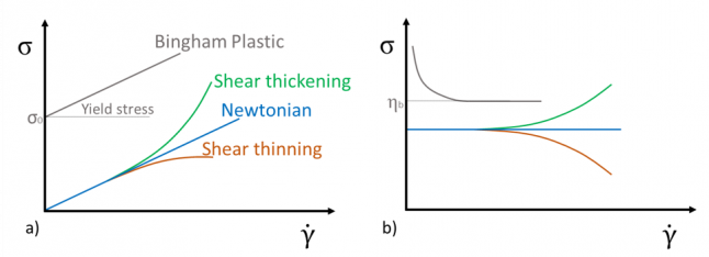
Figure 1. Flow curves of Newtonian and non-Newtonian fluids: Shear stress, σ, (a) and shear viscosity, η, (b) as functions of the shear rate, γ˙.

Several mathematical expressions are available to describe these behaviors: the easiest one is the so-called Power law:

$\eta = K \dot{\gamma}^{n-1}$

(K being a constant and n the flow index). Depending on n, this model is able to reproduce the Newtonian (n=1), the shear thinning (n<1) and shear thickening (n>1) character of the material. However, it cannot reproduce the Newtonian plateau and is missing, thus, the transition between the Newtonian and non-Newtonian behavior of the same fluid. Despite this limitation, the power law model is often applied since the low shear rate behavior is not always of interest. For example, one can think of the calculation of the pressure drop along a tube, where the less important loss occurs in the middle of the channel, where $\dot{\gamma}=0$ . On the other hand, a constitutive equation for Bingham fluids is usually expressed as:

$\sigma=0$ if $\sigma < \sigma_0$

$\sigma=\sigma_0 + \eta_b\dot{\gamma}$ if $\sigma > \sigma_0$

where $\eta_b$ is a parameter characterized by the dimensions of a viscosity and can depend on the flow conditions. In Figure 1b, $\eta_b$ is shown as constant: this means that, in the region where the Bingham material flows, it behaves like a Newtonian fluid, but this is not always the case ^[1].

[1] Macosko, C.W. (1996) Rheology: Principles, measurements, and applications, Wiley.com. Available at: https://www.wiley.com/en-us/Rheology%3A+Principles%2C+Measurements%2C+and+Applications-p-9780471185758 (Accessed: January 4, 2023).

Previous Chapter Next Chapter