LS Instruments | Maxwell model

Maxwell model

Dynamical and structural parameters of a sample provided by rheology can be described and quantified by mathematical models. The most simple and fundamental is the Maxwell model [1,2].

Figure 1. Maxwell unit.

It considers both the elastic and the viscous moduli of the material by assuming that the rheological properties can be represented by a spring and a dashpot connected in series. The former represents the elastic component and the latter the vicious one. In the Maxwell model, the elastic stress in the spring, σe, and the viscous stress in the dashpot, σν, are the same, whereas the strain of the system, γ, is the sum of the individual strains. Thus:

$\sigma = \sigma _e=G \gamma _e= \sigma _ \nu = \eta \dot{ \gamma } _ \nu$ (1)

$\gamma = \gamma _e+ \gamma _ \nu$ (2)

The constitutive equation for the Maxwell model is obtained by deriving eq. (2) and combining it with eq. (1):

$\dot{ \gamma }= \dot{ \gamma }_e+ \dot{ \gamma }_ \nu =\frac{1}{G}\frac{d \sigma }{dt}+ \frac{1}{ \eta } \sigma$ (3)

$\eta \dot{ \gamma }= \tau \frac{d \sigma }{dt}+\sigma$ (4)

where τis the relaxation time of the material. It is obtained as the ratio between the viscosity, η, and the shear modulus, G. The relaxation time $\tau$ gives you an indication of how long it takes a viscoelastic material to flow. In the case of an oscillatory motion, it is possible to formulate the constitutive equation:

$\frac{ \sigma }{ \gamma _0}=G' \sin( \omega t)+G'' \cos( \omega t)$ (5)

where

$G'=G\frac{ (\omega \tau)^2}{1+(\omega \tau)^2}$

$G''=G\frac{ (\omega \tau)}{1+(\omega \tau)^2}$ (6)

The typical Maxwellian oscillatory response is shown in Figure 2:

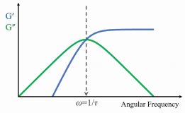
Figure 2. Sketch of a typical Maxwellian oscillatory response in a double logarithmic scale.

At very low frequencies, G″ is much larger than G′ and, hence, a liquid-like behavior predominates. However, as the testing frequency is increased, G′ takes over and solid-like behavior prevails. When G″ reaches a maximum G′ is equal to G″. This is the critical crossover frequency, which is the inverse of the relaxation time, $\tau$ .

Furthermore, at sufficiently low frequencies $\Big( \omega<<\frac{1}{\tau} \Big)$ , storage, and loss moduli in eq. (6) reduce to:

$G'=G_0( \omega \tau )^2$

$G''= \eta \, \omega$

This means that in a double logarithmic plot, in the so-called terminal region, G′ and G″ increase linearly with ω with slope 2 and 1, respectively. The Maxwell model is thus an easy mathematical approach to describe the rheological properties of many materials. However, it is worth noting that this is only one of the numerous models available for quantitative data analysis. The strength, as well as the weakness of the Maxwell Model, lies in its simplicity.

[1] C.W. Macosko, Rheology: Principles, Measurements and Applications, VCH Publishers, New York 1994.
[2] J.D. Ferry, Viscoelastic properties of polymers, 3rd Edition, Wiley, New York 1980.

Previous Chapter Next Chapter